

Analysis of the Earned Schedule Forecasting Accuracy
by Keight Charles Navarro Hurtado, PE PSP
Abstract–The independent estimate at completion (IEAC) is a time-based earned schedule (ES) method that allows the analyst to estimate the duration of a project according to the information available for a period of time. The fact that there are two approved equations that may give different results hinders the acceptance of this important analysis.
The purpose of this paper is to describe the two equations and determine which is more accurate to estimate the final duration of a project. In this analysis, the average absolute percentage error, completed percentage, seriality of the network diagram and productivity index (PI) have been used to evaluate the accuracy of the two equations.
A study of eight real projects with early and late completion will be used to determine the accuracy of each method. The conclusion is that when the schedule performance index based on the time is less than 1 or the project has a delay, the equation of the IEAC with the PF=1 begins to lose accuracy and the equation of the IEAC with the SPI begins to gain accuracy or has fewer errors.
Introduction
The time-based independent estimate at completion is an indicator that allows estimating the final duration of a project for an early or late completion. The IEAC has two methods to predict the duration. This work analyzes and determines which equation of the IEAC is more accurate throughout the life cycle of the project. In addition, a contrast will be made with the analysis of the writer Lipke [5], who dealt with the earned schedule forecasting method selection, its two forecasting methods and an optimum selection.
Case Study
This case study is the analysis of eight real construction projects of an oil refinery with an evaluation and accuracy of the two IEAC forecasts through the simple formula and the more general formula IEAC. Both forecasts allow one to estimate the total duration of a project. This paper will verify which of the two forecasts have a greater precision in the estimation of the total duration of a project. Better precision will help create a better estimate of the date of completion of the project. The two IEAC forecasts to be evaluated are the schedule performance index (SPI) and the equation with PF=1. The term PF=1 means the performance factor or future execution efficiency, which is used in the more general equation of the IEAC.
Methodology
The study begins with the calculation of the percentage error in each period of the project. This indicator allows evaluation of the degree of error in the forecasting of the IEAC with SPI and PF=1. Therefore, its purpose is to calculate the percentage error and observe the variations in the accuracy of the forecasts in the projects analyzed, once the percentage errors have been obtained.
The analysis continues with the calculation of the mean absolute percentage error (MAPE). Its formula is furnished in Appendix A, fig. 01 where the “RD” value means the actual duration of the project and the “Ft” value is the estimated forecasting of the IEAC in each period calculated for the analysis. In the study, the lowest MAPE calculated in both equations of the IEAC will be used as the more accurate method. Another parameter analyzed is the percentage completed. This factor impacts the evolution of the IEAC through the schedule performance index and, in addition, the percentage completed will allow the reader to observe its influence on the IEAC forecasts in each phase of the project.
In the study of the percentage completed with the MAPE, three phases are considered. The early phase is in the range of 0% ≤PC <30%, the intermediate phase in the range of 30% ≤PC ≤70% and the late phase in the range of 70% <PC≤100%
Another factor to consider in the impact of the IEAC forecast is the seriality. Seriality refers to the topology of the project network diagram. The study of the seriality with the MAPE has the following intervals to categorize the topology of the network diagram. If the network diagram is in parallel, the range is 0% ≤SP<40%, in series-parallel the interval is 40%≤SP≤60% and in series, its interval is 60% <SP≤100%. In the study, seriality is observed in two phases for analysis at the beginning of the project and at the end. This will help in understanding how the topology of the network diagram of the project changes towards its completion and how this change can impact the IEAC forecasts.
Another factor to consider is the index productivity. It will be used to evaluate the performance and its relationship with accurate IEAC forecasting through the observations in the IEAC analysis. The IEAC forecasting changes when low index productivity is high or low.
To understand how these change in the accurate forecasting occur, the SPI and ES of the earned schedule, as obtained, will be plotted through their natural logarithms and the standard deviation of the Ln (ES (t)). This will allow obtaining a range of intervals when the SPI is more accurate that the PF=1. The same happens with a range of intervals obtained when the PF=1 is more accurate than the SPI. These intervals will be used to calculate the forecasts and make a comparison with the real forecasts (the periods in which the SPI and the PF=1 are used depends on the MAPE).
Result
The result section summarizes the data of the methodology used. It contains the calculation of the MAPE, percent complete, seriality and productivity index.
MAPE
The results of the absolute average percentage errors made to the eight sample projects are shown in Table 01, along with %Error SPI and PF=1 in the early, intermediate and late phases of the eight projects.
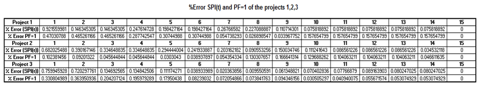
Table 1
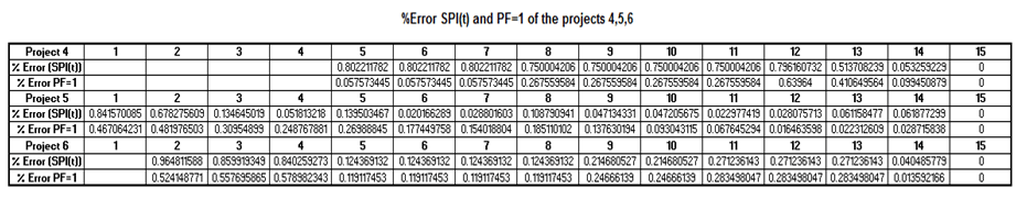
Table 2
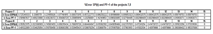
Table 3
In Tables 01, 02 and 03, the reader can see the summary of all the average absolute percentage errors calculated in the eight projects. As can be observed, PF=1 is the most accurate at the beginning of the project in all the eight projects. It can also be observed that the error changes as the project continues towards its completion. This change is the result of two important parameters. When the delay and productivity have been calculated and analyzed, there are considerations, as mentioned below:
- When there is a delay and low productivity in terms of the performance index SPI, the forecast of the IEAC with SPI is more accurate than PF=1.
- When there is a delay and high productivity in terms of the performance index SPI, the forecast of the IEAC with PF=1 is more accurate than SPI.
In Table 04, MAPE Summary of PF=1 Calculations, the reader can see the difference of error between the SPI and the PF=1 in 15 periods of analysis and also check the two considerations previously indicated.
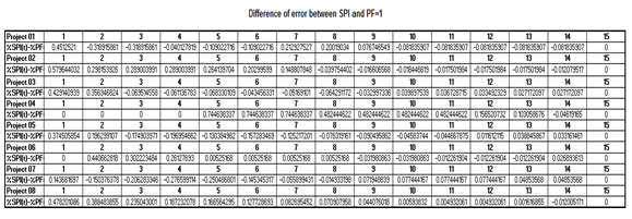
Table 4
Table 05 shows the MAPE summary of the eight projects analyzed. It is also observed that the forecast with the PF=1 is more accurate than that with SPI in six of the eight projects analyzed, while two reflect greater accuracy of the SPI forecast. It is also important to specify that only three projects out of the eight were completed early, viz., projects 01, 02 and 04.
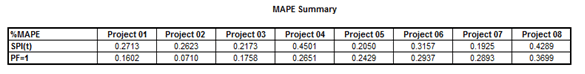
Table 5
Percent Complete (PC)
Table 06 shows the calculated values of the SPI and the PF=1 in the early, intermediate and late phases of the eight projects.
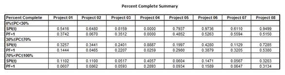
Table 6
Readers can see in the Table #06 the forecast of the IEAC with SPI and PF=1. The forecast with PF=1 is more accurate in the early phase of the eight projects. However, in the intermediate phase, six of the eight projects were more accurate with PF=1, but this change of accuracy in the PF=1 occurs in the intermediate phase of the projects #5 and #7. In the revised data of the projects #5 and #7, the forecast with SPI is more accurate than PF=1 and it occurs in the range of 0.1 and -0.6 of the natural logarithmic of the SPI. Reader can confirm the accuracy of the SPI from the following table with the data of the projects 05 and 07. All these values relate to the intermediate phase of both the projects.
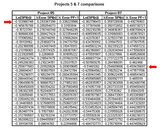
Table 7
In the late phase, some projects changed their accuracy with respect to the intermediate phase. This can be seen from Table 08 of the projects #3 and #6 and it occurs for the schedule performance index (SPI) or, in other words, for the productivity. For that reason, the forecast of the SPI is more accurate than that of the PF=1. The reader can observe the trend of the SPI in Table 06.
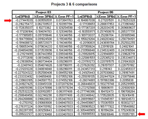
Table 8
Project Seriality (SP)
Seriality is an important concept to consider. It is the description of the structure of the project network, reflecting how close it is to a structure parallel, serial-parallel or serial. This topology structure of the network diagram varies from the beginning of a project until its completion. This change is due to the delay in the project. Table 07 shows the seriality at the start and end of each project and the MAPE of the forecasts with SPI and PF=1.
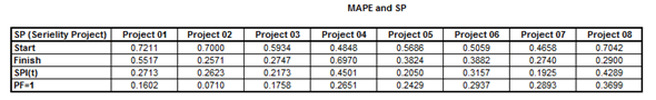
Table 9
In Table 09, the reader can see that project #1 started with a seriality in serial and ended with a seriality in parallel-serial. In all the life cycle of the same, the forecast with the PF=1 was more accurate than the SPI, and this project was completed early. Project #2 started with a seriality in series and ended in parallel, and in all the life cycle of the same, the forecast PF=1 was more accurate than the forecast SPI, and it was completed early. Project 03 started with a seriality series-parallel and ended in parallel, and in all the life cycle of the same, the forecast PF=1 was more accurate than the forecast SPI, and it was completed late. Project 04 started with a seriality series-parallel and finished with a seriality in series and was completed late. In this project, the forecast with PF=1 was more accurate than the SPI. Projects 05, 06, 07 and 08 had a delayed completion, and the accuracy of their forecasts were SPI, PF=1, SPI and PF=1, respectively. Readers may question why and when this change happens. As indicated earlier, the replies to these questions depend on the performance index of the SPI, which will be explained in this paper.
Productivity Index (PI)
In the analysis of the forecast of the earned schedule, the PI (index productivity) is also analyzed. Readers can see in Table 10 the index productivity of the eight projects with the average absolute percentage errors (MAPE) of the forecasts through SPI and PF=1. Project #1 has a PI of 0.7987 and its forecast with PF=1 is more accurate than the forecast with SPI. Project #3 has a PI of 0.7042 and its forecast with PF=1 is more accurate than the forecast with SPI. Project 05 has a PI of 0.6069 and its forecast with SPI is more accurate than the forecast with PF=1. The analysis of all the data indicates that there is no relationship between the PI and the performance index of the SPI. Hence, there is no link between the forecasts of the IEAC and the productivity index.
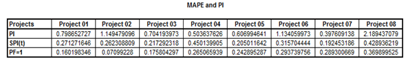
Table 10
Ln(SPI) and σLn(ES(t)) are analyzed in this section of the paper. This is done to have a compression above the accuracy of the forecasts as explained in the MAPE, PC, Seriality and PI and about the relationship with them of the performance index SPI.
In Figure 1, the reader can see the values of the six projects where the PF=1 was more accurate than the forecast SPI. These values were obtained from the calculation of the MAPE. In the observations, the values of the ln (SPI) are between 0.1 and 0.6, and if the values of the ln (SPI) are greater than 0.6, these values will be out of control. The reader can see in Fig.01 the values of the σLn (ES (t)) are in the range of 0.0 and 0.5.
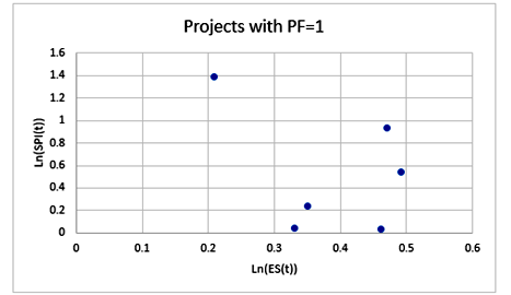
Figure 1–Projections using PF=1
Figure 2 shows the values of two projects where the forecast with the SPI is more accurate than PF=1. These values were obtained from the MAPE. The range of accuracy of the forecast SPI is between -0.1 and -0.6, but the analysis of the data of all the values of the Ln(SPI) shows a transition period, where the accuracy of forecast of the IEAC with the PF=1 changes from more to less, and the forecast with the SPI changes from less to more. This transition period occurs in projects with late completion. The interval of the transition period is between 0.1>Ln(SPI) and Ln(SPI)<-0.1. Hence, from the intervals described earlier in this section, it can be concluded that the interval of the SPI is between 0.1 and -0.6. If in the analysis of the data, values of the ln (SPI) are greater than -0.6, it will be considered out of control. The reader can see in Fig.02 the Ln (ES) is in the range of 0.0 and 0.5. The answers to the questions that arose previously when the seriality was analyzed are as follows. The change of accuracy of one forecast vis-à-vis the other happens when there is delay in the project, and it has a low productivity or high productivity in terms of the performance index SPI. This will happen in the intervals analyzed to the case of the PF=1, its interval being 0.1≤Ln(SPI) ≤0.6 and 0.5≤σLn (SPI), and in the case of the SPI, 0.1<Ln( SPI≤-0.6 and 0.5≤σLn (SPI).
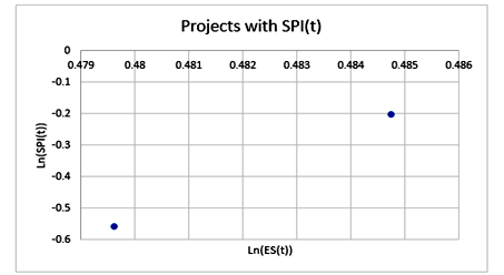
Figure 2–Projections of SPI
In addition, it is important to indicate that there are five projects with late completion, of which two reflect accuracy of the forecast SPI and three with the PF=1. Why does this happen? The answer is in the observations derived from the data: it happens when the project has a tendency in which the Ln(SPI)<-0.4 and a low productivity. Hence the forecast with SPI is more accurate than the forecast with PF=1, as can be observed in Figure 3.
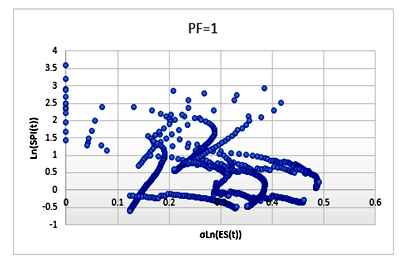
Figure 3
Figure 3 shows all the values of the six projects with the PF=1. There are values where the natural logarithmic exceeds -0.4 in some periods, so in this case, the PF=1 is more accurate. Because its productivity in terms of the SPI has been high, this raises the accuracy of the PF=1. It also consolidates the lower error in the MAPE, compared to the forecast of the SPI.
In Figure 4, all the values where the SPI is more accurate than the forecast of the PF=1 are furnished. These values have a tendency where the Ln (SPI)<-0.4. In this case, these projects had a low productivity and they have been delayed. Hence these projects had a low productivity in terms of the SPI plus delay, resulting in a lower error MAPE with the forecast through SPI with respect to PF = 1.
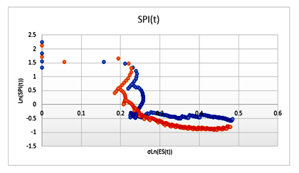
Figure 4
Walt Lipke made this analysis in his paper Earned Schedule Forecasting Method Selection and he lists below his selection rules for the forecast of the IEAC with the SPI and PF=1.
Use PF=1 when -0.1≤lnSPI≤0.1 and lnESpσ≤0.8
Use SPI when lnSPI>0.1 or < -0.1 and lnESpσ≤0.8
Use SPI when lnSPI≤0.6 or ≥-0.6 and lnESpσ≤0.8
Use PF=1 when -0.6>lnSPI>0.6 or lnESpσ>0.8 = Out of Control
The reader can see in Table 11 a comparative listing of the SPI, PF=1, Real, Calculating and Lipke.
Table 11
The values of the selection rule of Lipke have been compared with the other values in the same table, to calculate the accuracy grade of the intervals. MAPE of the observations in the SPI and PF=1 are given in the table. The range of intervals to the forecast of the IEAC with the PF=1 is 0.1≤ln (SPI) ≤1.0 and 0.5≤σln (ES). However, in the case of the forecast of the IEAC with the SPI, its range is between the intervals 0.1> ln(SPI)>-0.6 and 0.5≤σln (ES). In the same table, the reader can see that Real MAPE is lowest MAPE of all the values and that the calculated MAPE and Lipke are closer to the real values. The reader can see in Table 12 the difference between calculated and Lipke MAPE.
Table 12
The calculated MAPE and Lipke’s are closer to the real figure. However, of the two the calculated MAPE are closer to the real and Lipke has one project near the real MAPE.
Conclusion
The analysis performed with the MAPE, Percent Complete, Seriality and Index to the forecast of the IEAC resulted in PF=1 emerging with the highest accuracy. The productivity index as a factor of analysis of the accuracy about the forecasts of the earned schedule did not show a relationship with the forecast of the IEAC.
The forecasts of the IEAC have a logarithmic tendency.
From an objective point of view, the accuracy of the forecasts has been estimated in intervals to know when each forecast is more accurate.
The evaluation of the forecast of the IEAC with PF=1 and the SPI has been made with the natural logarithm.
The interval of the forecast of the IEAC with PF=1 is 0.1≤ln(SPI)≤1.0 and 0.5≤σln (ES).
The interval of the forecast of the IEAC with SPI (t) is 0.1> ln(SPI)>-0.6 and 0.5≤σln (ES).
There are periods in the projects where the values have a tendency towards the accuracy of the SPI due to the delay. However, when calculating the MAPE of that project, its accuracy is better with PF=1. This occurs due to the high productivity in terms of the performance index SPI. The same scenario occurs with the PF=1 too. There are periods in the projects when the values have a tendency towards the accuracy of the PF=1. While calculating the MAPE of the project, SPI displays more accuracy, which is due to low productivity in terms of the performance index SPI.
Only six projects have been covered here, so the analysis is based on limited data.
References
- Dr. Scott J. Amos, PE., Skill and Knowledge of Cost Engineering, 5th edition, AACE International, Morgantown, WV, 2007.
- James A. Bent and Kenneth K. Humphreys, Effective Project Management Through Applied Cost and Schedule Control, Marcel Dekker, New York 1996.
- Forrest D. Clark and A. B. Lorenzoni, Applied Cost Engineering, 3rd edition, Marcel Dekker, New York 1997.
- Dr. Frederic C. Jelen, Dr. James H. Black and Dr. Aaron Rose, Jelen’s Cost and Optimization Engineering third edition, AACE International, Morgantown, WV, 2013.
- Lipke, Walt. “Earned Schedule Forecasting Method Selection”, PM World Journal, January 2019, Vol. VIII, Issue I.
- Lipke, Walt. “Forecasting Schedule Variance Using Earned Schedule”, PM World Journal, February 2017, Vol. VI, Issue II.
- Jordy Batselier and Mario Vankhoucke, “Empirical Evaluation of Earned Value Management Forecasting Accuracy for Time and Cost”, ASCE 2015.
- Mario Vankhoucke, Measuring Time Improving Project Performance Using Earned Value Management, Springer, New York 2009.
- Quentin W. Fleming and Joel M. Koppelman, AACE International’s Professional Practice Guide to Earned Value Project Management.
- Dr. Joseph J. Orczyk, PE., Productivity, Analyzing Construction Productivity, AACE International, Morgantown, WV.
- Anghel Patrascu, Construction Cost Engineering Handbook, Marcel Dekker, New York 1988.
Appendix A
Earned Schedule
Earned schedule (ES) is a method that uses the earned value elements available based on duration variance, to calculate the performance and schedule variations. The results can be used to predict the total duration of the project in time units. The theory of the ES focuses on the time in which the earned value must have occurred.
ES is calculated from the formula:
ES = C + I
Equation 1
Where,
C = Earned Value but satisfying the condition EV ≥ PVn
I = Linear interpolation
“C” is determined by comparing the EV with the periodic values for PV. For example, PVn. “C” is the highest value of “n” that satisfies the condition, EV ≥ PVn. “I” is an interpolation using the equation:
I = (EV – PVC) / (PVC+1 – PVC)
Equation 2
Where,
C = Value progress time
I = Linear interpolation
Indicators of the Earned Schedule (ES)
The indicators of the earned schedule are the variation of the schedule (SV (t)) and the schedule performance index (SPI(t)). The equations are determined by the following:
SV(t) = ES – AT
Equation 3
SPI(t) = ES / AT
Equation 4
Where “AT” is the actual time, for example from the beginning until the EV is measured
Independent Estimate at Completion (time)
This indicator estimate the completion of the project and there are two methods of calculating it. The simple form is:
IEAC = PD/SPI
Equation 5
And the more general form is:
IEAC = AT + (PD-ES)/PF
Equation 6
Mean Absolute Error
The mean absolute percentage error (MAPE) is a statistical measure of how accurate a forecast system is. It measures this accuracy as a percentage and can be calculated as the average absolute percent error for each time period minus actual values divided by actual values.

Equation 7
Where,
At= The actual value
Ft= The forecast value
n= Period numbers
Percent Complete
The completed percentage enables measurement and analysis of productivity and measurement of the completed percentage of work activities. There are six methods in this regard:
1. Units Completed
2. Incremental Milestone
3. Start/Finish Percentages
4. Ratio
5. Supervisor Opinion
6. Weighted or Equivalent Units
Seriality
The seriality is the topological network diagram and is directly linked to the number of critical activities in a network.
Index Productivity
The productivity index consists of the credit workhours and the actual hours. The PI is calculated through the following formula.
PI = Credit Workhours/Actual hours
Equation 8
Table and Figure Image Details.
Click on any image to launch widget.
Rate this post
Click on a star to rate it!
Average rating 4.9 / 5. Vote count: 9
No votes so far! Be the first to rate this post.
Interesting paper, Keight that will be required reading by all my students.
Check out the work that Steve Patterson has done on this topic?
https://pmworldlibrary.net/wp-content/uploads/2018/01/pmwj66-Jan2018-Paterson-comparison-of-8-common-forecasting-methods-featured-paper.pdf
This paper may also be of interest to you as at least some of us “old timers” swear that “Earned Time” or “Earned Schedule” has always been a key component of Earned Value Management.
https://pmworldlibrary.net/article/the-origins-and-history-of-earned-value-management-a-contractors-perspective/
just need a case with numbers to show how to use each Equation
It is always great to come across a page where the admin take an actual effort to generate a really good article. Check out my website 94N concerning about Content Writing.